A. Aleksiev*, B. Kostova and D. Rachev
Department of Pharmaceutical Technology and Biopharmaceutics, Medical University-Sofia, Faculty of Pharmacy, 2 Dunav str., 1000 Sofia, Bulgaria
- *Corresponding Author:
- A. Aleksiev
Department of Pharmaceutical Technology and Biopharmaceutics, Medical University-Sofia
Faculty of Pharmacy, 2 Dunav str., 1000 Sofia, Bulgaria
E-mail: angelaleksiev@yahoo.com
Received date: 10 Dec 2015; Revised date: 01 Jun 2016; Accepted date: 12 Jun 2016
Abstract
This study is focused on the development and optimization of the reservoir-type oral multiparticulate drug delivery systems loaded with galantamine hydrobromide. For this purpose, the process of applying of the drug onto sugar pellets through the medium of a hydroxypropyl methylcellulose-based suspension was investigated. A substantial part of the study was to refine the layering process in respect to the influence of critical process parameters on the formation of agglomerates between the pellets. This outcome is related to some critical coating factors, such as: spray rate, product temperature, airflow, concentration of hydroxypropyl methylcellulose in the coating suspension and spray pressure. In this study design of experiments was used as a statistical method for assessing the influence of critical process parameters on the agglomeration. For this purpose full factorial design of five factors at two levels was built. The effect of the main factors and their interaction on the response was evaluated using regression analysis, analysis of variance and graphical analysis of the experimental design. The results showed that the airflow and the concentration of hydroxypropyl methylcellulose in the coating suspension have the most significant effect on the formation of agglomerates during the drug layering process.
Keywords
Design of experiments, full factorial design, drug layering, fluid bed system, galantamine hydrobromide
Improving the quality of drug delivery systems and the efficiency of the manufacturing process are the main priorities of the modern pharmaceutical industry. In this respect the optimization of the production of reservoir-type oral multiparticulate drug delivery systems is a serious technological challenge[1]. The problem is in the fact that the drug layering is extremely vulnerable as regards the variations of the process parameters. The difficulty comes from the reality that conditions are created for forming agglomerates of pellets, due to sticking to one another. The formation of agglomerates causes reduction of the total surface area for the subsequent applying of a polymeric membrane and consequently alters the drug dissolution profile. Furthermore, it makes difficult for the proper dosage of the pellets in the final dosage form and it worsens uniformity of mass and uniformity of drug content of the product as well. The possibility of forming agglomerates could be controlled through a precise analysis of the influence of process parameters whose detailed differentiation would be an important step in the optimization of production processes and is a major factor in ensuring the quality of the drug product.
The conditions of the pellet coating technological process are determined by different input variables, which are the so-called critical process parameters (CPP). CPPs are the independent variable factors whose variation affects the final result of the process. An important step in the Quality by design (QbD) is determining the impact of the CPPs on the quality of the product defined on the basis of the critical quality attributes (CQA). The statistical tools, such as the design of the experiment (DOE), which include screening, and response surface models, and multicriteria decision methods (MCDM) help to achieve this goal[2,3].
DOE is a useful organized method for planning experiments, whose object is to determine the impact (effect) of the CPPs of a given process on the tested critical parameter of the product (response) with minimum experiments. For each experiment the result is measured and the ordinary least squares (OLS) regression, known as multiple linear regression (MLR), is used in order that the relationship between the factors and the response should be identified[4,5]. Once the relation is identified, the process can be mathematically optimized by choosing the best combination of parameters for the achievement of certain goals.
One of the active ingredients which is of interest to be included in reservoir coated multiparticle delivery systems is the cholinesterase inhibitor galantamine hydrobromide. It is a reversible, competitive inhibitor of the enzyme acetylcholinesterase whose main indication is the treatment of mild to moderate dementia in people with Alzheimer’s disease, at a dose of 16-24 mg per day[6-9]. Galanthamine hydrobromide is a weak base with 90% oral bioavailability after oral administration, and the time to reach the maximum plasma concentration (tmax) is approximately 1 h[10]. According to the Biopharmaceutics Classification System (BCS), galantamine hydrobromide belongs to class I i.e. drugs with high solubility and high permeability[11].
The purpose of this study is to be focused in detail, through the use of DOE and various statistical methods, on the study of the impact (effect) of the CPPs in the layering of sugar pellets with a hydroxypropyl methylcellulose (HPMC)-based suspension of galanthamine hydrobromide on the forming of agglomerates. Thus, by differentiation of the significance of the effects of various factors on the degree of agglomeration, should be optimized, and the quality of the obtained product will be guaranteed.
Materials And Methods
Galantamine hydrobromide (Sopharma AD, Bulgaria), HPMC, nominal viscosity of 5 mPa.s (Methocel® E5 Premium LV, Dow Chemical Co., USA), sugar spheres with particle size range of 850-1000 microns (Suglets®, Colorcon, England), glycerol monostearate 40-55 type I (Geleol®, Gattefossé, France), polyethylene glycol (PEG) 400 (Polyglycol® 400, Clariant Produkte GmbH, Germany). All substances were obtained as a gift sample from Sopharma AD, Bulgaria.
Obtaining of coated pellets loaded with galantamine hydrobromide:
For obtaining the coated pellets, standard sugar spheres with a nominal diameter of 850-1000 μm were used. The coating was done using an aqueous suspension of galantamine hydrobromide HPMC, PEG 400 and glycerol monostearate. Single dosage unit consists 30.77 mg of galantamine hydrobromide, which is equivalent to 24 mg galantamine base. The coating of the spheres was carried out in Oystar Huttlin Unilab laboratory fluid bed system (Huttlin GmbH, Germany), provided with nozzles for bottom spraying with 1.2 mm diameter. Once the coating was completed the pellets were taken out and allowed to remain at room temperature for 2 h, immediately thereafter, they were analyzed for the content of the obtained agglomerates.
Sieve analysis of pellets:
A sieve shaker (Vibro, Retsch GmbH, Haan, Germany) provided with mesh sized sieves of 1.4, 1.25, 1.12, 1.0 and 0.63 mm was used. For border size sieve sized 1.25 mm was fixed. The analysis was performed with 100 g of coated pellets for 15 min with amplitude of the sieve of 1.5 mm. Results were expressed as a percentage of pellets retained over a sieve sized 1.25 mm.
Design of the experiment:
Full factorial design for five factors at two levels (25) was carried out to evaluate the effects of five process factors: spray rate and spray pressure of the nozzle, product temperature, airflow, and HPMC concentration in the suspension for coating on the response, i.e. the percentage of agglomerates being obtained. Each factor was set at two levels which were given as high and low, coded as (-1) and (+1), respectively. Following the typical practice for two level designs, we included three replicated center points coded as (0). The addition of center points allows an independent estimate of the error to be obtained without affecting the estimated of the factorial effects. Using these center points gives the possibility to verify if there is a non-linear component in the relationship between the individual factor and the dependent variable. They serve as a measure for the stability of the processes at the specified levels of the variable factors, as well as to check the curvature.
Determination of the effect of the variable factors on the response:
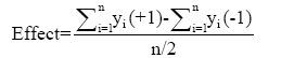
The main calculations which are included in the first steps of analyzing the experimental design are the determination of factor effect and t-value of the effect[12]. The effect of one factor on the response is calculated according to Eqn. 1,
 (1)
(1)
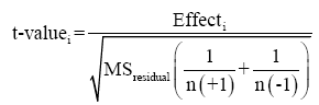
Where, n is the number of the experimental points at each level, and y is the respective response for each point. The t-value of the effect is mathematically determined according to Eqn. 2,
 (2)
(2)
Where, n is the number of responses from each of the two studied levels (-1 and +1), and MSresidual is mean square of the residuals calculated by Analysis of variance (ANOVA). Based on the results of t-values a Pareto plot of factor effects and a normal probability plot of factor effects were drawn.
The experimental design was analyzed by use of an ANOVA, which estimates the statistical significance of a factor or a group of factors on the response. Sums of squares (SS), degrees of freedom (df), mean squares (MS), mean square error (MSE), F-value, ?-value, lackof- fit, coefficient of determination (R2) and adjusted coefficient of determination (adj. R2) were included in the analysis. The calculations were made with a 90 % confidence interval and a significance level α=0.05[13].
Graphical analysis of the experimental design:
Interaction plots, a response surface plot, a normal probability plot of the residuals and a plot of residuals versus corresponding predicted values were used as graphical tools for analysis of the factorial design.
Regression analysis:
A regression analysis was used to illustrate the mathematical relationship between the independent variables and the response. By means of it the response could be predicted with different combinations of the process parameters at its most efficient levels[14]. The experimental data were processed by use of software STATISTICA version 10 (StatSoft, Inc., USA).
Results And Discussion
About 300 g of sugar pellets were coated with aqueous dispersion containing 30.0 g of HPMC, 9.0 g of PEG 400 and 3.0 g of glycerol monostearate. Each sample was provided for the preparation of 1000 dosage units, each of them containing 30.77 mg galanthamine hydrobromide (equivalent to 24.0 mg of galantamine base). All experiments were carried out with the same qualitative and quantitative ratio of the final composition. After drying, the coated pellets were analyzed for determining the percentage of agglomerates.
In our preliminary studies on the process of coating of sugar pellets with a suspension of galanthamine hydrobromide was specified that five factors have a critical impact on the degree of agglomeration of the pellets. They are spray rate (?), product temperature (?), airflow (?), HPMC concentration in the suspension for coating (D) and spray pressure (E). These five factors were studied in the experimental design at two levels: low (-1) and high (+1). Each value of the low level was ? of the value of the high level. Three center points (cp) were added in design, which level was the average of the high and the low level of the main factors. These three additional experiments were codded as (0). The five factors, the three replicated center points, and the units are represented in Table 1.
| Factors | Name of the process factor | Unit | Low level (-1) |
Center point (0) |
High level (+1) |
|---|---|---|---|---|---|
| A | Spray rate | g/min | 3.6 | 4.5 | 5.4 |
| B | Product temperature | ° | 30 | 37.5 | 45 |
| C | Airflow | m3/h | 100 | 125 | 150 |
| D | HPMC concentration | % | 10 | 12.5 | 15 |
| E | Spray pressure | atm | 0.5 | 0.625 | 0.75 |
TABLE 1: FACTORS AND LEVELS
A matrix of full factorial design based on the represented five factors at two levels (25) and three central points was built. All combinations with the levels of the factors are represented in Table 2. Each combination was experimentally processed. The experiments were carried out in a randomized sequence in order to meet the statistical requirement for independence of the observations. The pellets obtained were examined for percentage content of agglomerates – response (Y). The obtained response data are represented in Table 2.
| Run order | Standard order | Spray rate (g/min) | Product temp.(°) | Airflow (m3/h) | HPMC (%) |
Spray pressure (atm) |
Y:Content of agglomerates (%) |
|---|---|---|---|---|---|---|---|
| 1 | 27 | −1 | +1 | −1 | +1 | +1 | 53.9 |
| 2 | 33 (?p)* | 0 | 0 | 0 | 0 | 0 | 52.1 |
| 3 | 14 | +1 | −1 | +1 | +1 | −1 | 33.5 |
| 4 | 25 | −1 | −1 | −1 | +1 | +1 | 85.3 |
| 5 | 15 | −1 | +1 | +1 | +1 | −1 | 43.5 |
| 6 | 26 | +1 | −1 | −1 | +1 | +1 | 93.6 |
| 7 | 18 | +1 | −1 | −1 | −1 | +1 | 61.6 |
| 8 | 34 (?p)* | 0 | 0 | 0 | 0 | 0 | 54.2 |
| 9 | 32 | +1 | +1 | +1 | +1 | +1 | 59.1 |
| 10 | 24 | +1 | +1 | +1 | −1 | +1 | 8.7 |
| 11 | 5 | −1 | −1 | +1 | −1 | −1 | 23.1 |
| 12 | 8 | +1 | +1 | +1 | −1 | −1 | 11.2 |
| 13 | 2 | +1 | −1 | −1 | −1 | −1 | 65.5 |
| 14 | 28 | +1 | +1 | −1 | +1 | +1 | 67.4 |
| 15 | 21 | −1 | −1 | +1 | −1 | +1 | 19.4 |
| 16 | 29 | −1 | −1 | +1 | +1 | +1 | 23.6 |
| 17 | 3 | −1 | +1 | −1 | −1 | −1 | 2.8 |
| 18 | 1 | −1 | −1 | −1 | −1 | −1 | 56.3 |
| 19 | 35 (?p)* | 0 | 0 | 0 | 0 | 0 | 48.5 |
| 20 | 20 | +1 | +1 | −1 | −1 | +1 | 39.8 |
| 21 | 17 | −1 | −1 | −1 | −1 | +1 | 53.2 |
| 22 | 19 | −1 | +1 | −1 | −1 | +1 | 2.3 |
| 23 | 16 | +1 | +1 | +1 | +1 | −1 | 61.1 |
| 24 | 4 | +1 | +1 | −1 | −1 | −1 | 42.9 |
| 25 | 22 | +1 | −1 | +1 | −1 | +1 | 60.6 |
| 26 | 30 | +1 | −1 | +1 | +1 | +1 | 33.8 |
| 27 | 10 | +1 | −1 | −1 | +1 | −1 | 94.1 |
| 28 | 23 | −1 | +1 | +1 | −1 | +1 | 1.2 |
| 29 | 12 | +1 | +1 | −1 | +1 | −1 | 69.6 |
| 30 | 11 | −1 | +1 | −1 | +1 | −1 | 57.3 |
| 31 | 31 | −1 | +1 | +1 | +1 | +1 | 39.9 |
| 32 | 6 | +1 | −1 | +1 | −1 | −1 | 62.2 |
| 33 | 13 | −1 | −1 | +1 | +1 | −1 | 26.2 |
| 34 | 7 | −1 | +1 | +1 | −1 | −1 | 1.6 |
| 35 | 9 | −1 | −1 | −1 | +1 | −1 | 84.3 |
*cp stands for central point
TABLE 2: MATRIX AND DATA FOR 25 FULL FACTORIAL DESIGN WITH CENTER POINTS
The effects of all main factors and their interactions up to level 3 on the response were calculated. At level 2, interactions were coded as AB, AC, AD, AE, BC, BD, BE. CD, CE and DE, and at level 3 were coded as ABC, ABD, ABE, BCD, BCE and CDE respectively. The choice to investigate the effect of the interactions only to level 3 was based on the fact that most of the processes are controlled by main factors and several interactions at a low level and most of the interactions at a higher level could be deemed insignificant[15]. Through ANOVA was determined the significance of the impact (F-ratio and P-value) of the main factors and their combination up to level 3. All obtained results are represented in Table 3.
| Effect | t-value | SS | df | MS | F-ratio | P-value | |
|---|---|---|---|---|---|---|---|
| Mean/Intercions | 44.956 | 29.662 | 0.000000 | ||||
| Curvature | 13.288 | 1.283 | 121.07 | 1 | 121.068 | 1.647 | 0.235 |
| (A) Spray rate | 18.175 | 5.996 | 2642.64 | 1 | 2642.645 | 35.951 | 0.000325* |
| (B) Product temperature | -19.625 | -6.474 | 3081.13 | 1 | 3081.125 | 41.917 | 0.000193* |
| (C) Airflow | -26.325 | -8.685 | 5544.04 | 1 | 5544.045 | 75.423 | 0.000024* |
| (D) HPMC concentration | 25.863 | 8.532 | 5350.95 | 1 | 5350.951 | 72.796 | 0.000027* |
| (E) Spray rate | -1.9875 | -0.656 | 31.60 | 1 | 31.601 | 0.430 | 0.530 |
| AB | 1.4875 | 0.491 | 17.70 | 1 | 17.701 | 0.241 | 0.637 |
| AC | 0.788 | 0.260 | 4.96 | 1 | 4.961 | 0.068 | 0.802 |
| AD | -5.900 | -1.946 | 278.48 | 1 | 278.480 | 3.789 | 0.088 |
| AE | 0.050 | 0.017 | 0.02 | 1 | 0.020 | 0.0003 | 0.987 |
| BC | 12.613 | 4.161 | 1272.60 | 1 | 1272.601 | 17.313 | 0.003161* |
| BD | 16.800 | 5.542 | 2257.92 | 1 | 2257.920 | 30.718 | 0.000546* |
| BE | -0.225 | -0.074 | 0.41 | 1 | 0.405 | 0.006 | 0.943 |
| CD | -9.275 | -3.060 | 688.20 | 1 | 688.205 | 9.363 | 0.015587* |
| CE | -0.025 | -0.008 | 0.00 | 1 | 0.005 | 0.00007 | 0.994 |
| DE | 0.363 | 0.120 | 1.05 | 1 | 1.051 | 0.014 | 0.908 |
| ABC | -6.975 | -2.301 | 389.21 | 1 | 389.205 | 5.295 | 0.050 |
| ABD | 1.888 | 0.623 | 28.50 | 1 | 28.501 | 0.388 | 0.551 |
| ABE | -0.288 | -0.095 | 0.66 | 1 | 0.661 | 0.009 | 0.927 |
| ACD | 0.513 | 0.169 | 2.10 | 1 | 2.101 | 0.029 | 0.870 |
| ACE | 0.513 | 0.169 | 2.10 | 1 | 2.101 | 0.029 | 0.870 |
| ADE | 0.475 | 0.157 | 1.81 | 1 | 1.805 | 0.025 | 0.879 |
| BCD | 11.838 | 3.905 | 1121.01 | 1 | 1121.011 | 15.251 | 0.004511* |
| BCE | 0.113 | 0.037 | 0.10 | 1 | 0.101 | 0.0014 | 0.971 |
| BDE | -0.950 | -0.313 | 7.22 | 1 | 7.220 | 0.098 | 0.762 |
| CDE | -0.325 | -0.107 | 0.84 | 1 | 0.845 | 0.012 | 0.917 |
| Model | 22846.34 | 26 | 878.705 | ||||
| Error | 588.05 | 8 | 73.506 | ||||
| Total SS | 23434.39 | 34 |
R2=0.97491 ; R2 adj=0.8933; SS is sum of squares, df is degree of freedom, MS is mean squares; *P-value<0.05 indicates significance.
TABLE 3: ESTIMATED EFFECTS AND ANOVA
From the values for Effect and t-value in Table 3 it could be assumed the force and the direction of impact of the main factors and their interactions on the formation of agglomerates. It could be seen that the greatest effect from the main factors have airflow (C) and the concentration of HPMC (D). Their effect on the response is –26.325 and 25.863, accordingly. Two other factors also demonstrated a high impact on the formation of agglomerates, namely: temperature of the product (B) and spray rate (A) with effect of –19.625 and 18.175, accordingly. The only main factor presenting a weak effect on the response was spray pressure (E), with a value of –1.987. From the interactions, a high effect showed the combinations: BD (16.80), BC (12.613), CD (–9.275) and BCD (11.838).
From the results presented in Table 3 it could be seen that two of the main parameters (A and D) have a positive effect, and the others (B, C and E) have a negative effect. This is due to the fact that with a change of the factor levels from low (-1) to high (+1) or opposite from high (+1) to low (-1) there is a relevant change in the percent of agglomerated pellets. Thus, factors with positive values of the effects (A and D), lead to an increase in the percentage of agglomerates. In contrast, factors with negative values (B, C and D), lead to a decrease in the quantity of agglomerates. The practical application of this statement is that a minimum quantity of agglomerates could be achieved when A and D are at a low level, and B, C and E are at a high level.
From ANOVA for the values of F-ratio and P-value, we assessed the statistical significance of the individual factors and their combinations on the response. These which reveal the most significant effect on the response, with a P-value less than 0.05 and high value of F-ratio are the main factors A, B, C and D, the interactions at two levels BC, BD, CD and the interaction at three levels BCD. The only main factor that it is statistically insignificant in regard to the response was E.
From the data in Table 3, regarding the general model we noted the following important characteristics: (i) the average P-value for the model is much less than 0.05, which indicate that the conditions in it have a high significance, which is also in accordance with the very high mean effect (44.956), (ii) Curvature has a P-value of 0.235, considerably above the level of significance, α=0.05, which means that it is statistically insignificant, i.e. there is a linear dependence between the response and the factors.
The coefficient of determination (R2) which shows the proportional variation in the response explained by the independent variables in the linear regression model is 0.975, and the adjusted coefficient of determination (R2adj) is 0.893. The value of R2, which is close to 1, reveals that there is a considerable linear relationship between the factors and the response. The value of R2 (0.975) demonstrates that with more than 97% confidence, the change in the response can be explained with the variables of the model. There is a slight difference between the R2 and R2 adj values, which shows that some insignificant conditions were included in the model.
A bar graphic, known as Pareto chart was used as a graphical representation for assessing the effects of the main factors and their interactions on the response sorted by their absolute size. Figure 1 shows the bars of the main factors and their combinations arranged in descending order according to the values of the standardized effect (t-values). With a vertical line is marked P-value (P=0.05), which is the statistical threshold for a level of significance. The bars which cross that line show that the main factors or their combinations have statistical significance on the response.

Fig. 1: Pareto chart of standardized effects.
From the results presented in the fig. 1 it can be clearly seen that four out of the five main factors have a statistically significant effect on the response. In a descending order according to their effect estimates they are: C, D, B and A. From the interactions, the following have a statistically significant effect: BD, BC, CD and BCD.
Another method for assessing the significance of the factor effects on the studied result is by use of a normal probability plot of factor effects. If the standardized effects represented by t-values demonstrate a weak effect on the response, they will assume a normal distribution and their values will lie on a straight line in the range close to zero. Values away from the straight line will show the considerable effect of an individual factor or combinations of factors on the response. The results are represented in fig. 2.

Fig. 2: Cumulative normal probability of effect estimates.
From the fig. 2, it could be seen that the standardized effects for more of the main factors and some of their combinations are not normally distributed on a line which is ranged close to zero. Four of the individual factors show a deviation of a varying degree – A, B, C and D, three of the combinations at level two – BD, BC and CD as well as the triple combination – BCD. All of them could be considered as more considerable regarding the impact on the response.
In order to determine whether two technological factors interact between themselves and what is the direction of this interaction, a method of graphic of interactions was used. Interaction is defined as inability of one factor to cause the same effect on the response with different levels of another factor[15]. Thus, there is an interaction between two variables when a change in the values of one variable alters the effect on another[16]. The change of the percentage of agglomerates (drawn on Y-axis) with a simultaneous change in the levels of the two factors graphically are presented as lines. If the lines are not parallel, the plot shows that there is an interaction between the factors. The highest the degree of deviation, the stronger is the effect of interaction[14]. With a statistical reliability it has already been shown that we observed significant interactions at two levels with combinations of the following factors: BC, BD and CD. In fig. 3 are represented the plots of the interaction between these factors.

Fig. 3: Interaction effect of factors on the % retained pellets.
The graphics of interaction on fig. 3 demonstrate nonparallel lines, which mean that there is an interaction between the factors. The graphics of the interaction between the temperature of the product and the airflow (fig 1a and 1b) show that the agglomeration of the pellets was lowest (about 28%) when the two factors were at a high level and it was highest when the two factors were at a low level (about 74%). The dependence between the product temperature and the concentration of HPMC (fig 2a and 2b) shows that the lowest quantity of agglomerates has been obtained when the first factor was at a high level, and the second one was at a low level (about 14%), and opposite: a highest quantity was obtained when the first factor is at a low level and the second one is at a high level (about 59%). Graphics of the interaction between the airflow and the concentration of HPMC (fig. 3a and 3b) demonstrate that there is lowest m agglomeration when the first factor was at a high level and the second one was at a low level (23.5%), and there was highest agglomeration when the first factor was at a high level, but the second one was at a high level (about 75.5%).
The data of the three independent central samples were used to test the lack-of-fit. The purpose of the analysis was to determine when the lack-of-fit error is comparable with the model error and whether it is at a level of significance, α=0.05. The test is also known as check for curvature for a factorial design at two levels[17]. The data of the analysis, according to ANOVA, are represented in Table 4.
| SS | df | MS | F-ratio | P-value | |
|---|---|---|---|---|---|
| Model | 22846.34 | 26 | 878.705 | ||
| Lack of fit | 571.43 | 6 | 95.238 | 11.4607 | 0.082415 |
| Pure error | 16.62 | 2 | 8.310 | ||
| Total SS | 23434.39 | 34 |
SS is sum of squares, df is degree of freedom, MS is mean squares
TABLE 4: LACK OF FIT
According to Table 4, a low value for the error of the model is obtained (SS=16.62) which determines good applicability with regards to the data. The results represented in the table show that the lack-of-lift has a P-value of 0.082, i.e. P>α, therefore it is statistically insignificant. That suggests that the dependence between the response and the independent variables is linear and the use of additional models for assessing the linearity is not necessary.
Response surface plot helps to establish the desired values of the response in the working conditions. In fig. 4 there is represented the 3D surface graphics for the mutual impact of two factors on the formation of agglomerates during the coating process. All possible combinations between the four significant factors (A, B, C and D) are assessed. For each presented plot, on the X and Y axis are mapped the two studied factors, and on the Z axis is presented the response. These plots visualize the expected response when random values of the two factors are admitted in the studied range from their low level (-1) to their high level (+1).

Fig. 4: 3D surface plots.
All panels show a lack of curvature in the surface profile according to the data in Table 3 where it could be seen that the curvature is insignificant (the P-value is 0.235). It could be noted that because of interactions between some of the factors (BC, BD, CD) the surface of response is in the form of a twisted plane.
The regression analysis illustrates the statistical relationship between one or more independent variables and the variable response and new observations could be predicted. By taking into account only the main factors and their combinations which demonstrated significant effect on the response a general equation can be obtained with regard to the real values by least square regression method. For predicting the percentage of agglomerates obtained, the following equation was derived:
Aggl% = 44.96 9.09A 9.81B 13.16C 12.93D + 6.31BC 8.40BD 4.64CD 5.92BCD
Where, A, B, C, D are the coefficients for the main process factors respectively, and BC, BD, CD and BCD are the coefficients values for corresponding interactions.
One of the main assumptions for the developed model is that the errors are normally distributed and they have constant variance. To check this statement, normal probability plot of residuals was used. The residuals are the differences in the values between experimental (observed) and predicted values of the response. If the residuals fall approximately on a straight line, they are considered as normally distributed and the model is adequate.
In fig. 5, a normal probability plot of residuals is presented for the values of the response. From the fig. 5, it can be clearly seen that all experimental values were very close to the theoretically expected ones (the straight line), which confirms the adequacy of the model. In fig. 6, a plot of the residuals versus the predicted values of the response is presented. The results presented in fig. 6 show that there is no characteristic model and unusual structure. The residuals are symmetrically positioned and tend to group in the low values of the Y-axis. There is a random distribution of the points around 0, which supported the statistical assumption for a constant variation. On the basis of the figs. 5 and 6, it could be assumed that the proposed model is adequate and there are no grounds for allowing violation of the independence or of the constant variation.

Fig. 5: Normal probability plot of residuals.

Fig. 6: Plot of the residuals versus predicted values of response.
Financial support and sponsorship:
Nil.
Conflicts of interest:
There are no conflicts of interest.
References
- Tallapaka SH, Karuturi VK, Sotthivirat S, Vetro JA. Controlled Drug Delivery. In: Mitra AK, Kwarta D, Vadlapudi AD, editors. Drug Delivery. 1st edition. Burlington: Jones and Bartlet Learning; 2015. p.108-28.
- Harrington EC. The Desirability Function. Ind Quality Control 1965;21:494-8 .
- Cox GM, Cochran W. Experimental Designs. 2ndedition. New York: John Wiley and Sons; 1957.
- Box GEP, Hunter WG, Hunter JS, Statistics for Experimenters. New York: John Wiley and Sons; 1978.
- Draper NR, Smith H. Applied Regression Analysis. 2ndedition. New York:John Wiley and Sons;1981.
- Jann MW, Shirley KL, Small GW. Clinical pharmacokinetics and pharmacodynamics of cholinesterase inhibitors. ClinPharmacokinet 2002;41:719-39.
- Robinson DM, Plosker GL. Galantamine extended release. CNS Drugs 2006;20:673-81.
- Abascal K, Yarknell E. Alzheimer's disease: Part 1 - Biology and botanicals. Alternat Complement Ther 2004;10:18-21.
- Lyseng-Williamson KA, Plosker GL. Spotlight on galantamine in Alzheimer's disease. Dis Manag Health Out 2003;11:125-8.
- Maltz MS, Kirschenbaum HL. Galantamine: A new acetylcholinesterase inhibitor for the treatment of Alzheimer's disease. P and T 2002;27:135-8.
- Drug label: REMINYL® (GalantamineHBr) tablets and oral solution. Food and Drug Administration; 2001.
- Anderson M, Whitcomb P. DOE Simplified: Practical Tools for Effective Experimentation. 2ndedition. New York: Productivity Press; 2007.
- Armstrong AN. Pharmaceutical Experimental Design and Interpretation. Bristol, PA: Taylor and Francis group; 2006.
- Antony J. Design of Experiments for Engineers and Scientists. Oxford: Elsevier Butterworth-Heinemann; 2006.
- Montgomery DC. Design and Analysis of Experiments. 7thedition. New York: John Wiley and Sons; 2009.
- Broota KD. Experimental Design in Behavioural Research. New York: John Wiley and Sons;1989.
- Wu CFJ, Hamada M. Experiments: Planning, Analysis and Parameter Design Optimization, 2ndedition. New York: John Wiley and Sons; 2000.